By the end of this chapter, you should be able to:
Explain the basic intuition of the gravity model of trade.
Identify why GDP and distance matter for bilateral trade flows.
Interpret the expected signs of common gravity variables.
Explain how trade costs affect bilateral trade.
Use a simple gravity-style equation to compare predicted trade across partners.
Connect gravity logic to regional trade agreements and TINA-style FTA simulations.
Why this chapter matters
Earlier chapters explained why countries trade using comparative advantage, factor endowments, and welfare analysis. The gravity model asks a different but very practical question:
Why does a country trade more with some partners than others?
The answer is usually not only comparative advantage. Trade also depends on the size of the partner economy, distance, transport costs, common borders, language, institutions, tariffs, and regional agreements.
For applied trade analysis, the gravity model is useful because it connects trade theory to observable country-pair data.
The basic idea
The gravity model is inspired by Newton’s law of gravity. In physics, the attraction between two objects increases with their mass and decreases with distance.
In trade economics, bilateral trade tends to increase with the economic size of the two countries and decrease with trade costs, especially distance.
A simple gravity-style expression is:
\[
Trade_{ij} = A \frac{GDP_i^{\alpha} GDP_j^{\beta}}{Distance_{ij}^{\gamma}}
\]
where:
\(Trade_{ij}\) is trade between country \(i\) and country \(j\),
\(GDP_i\) is the economic size of country \(i\),
\(GDP_j\) is the economic size of country \(j\),
\(Distance_{ij}\) is distance between the countries,
\(A\) is a scaling factor,
\(\alpha\), \(\beta\), and \(\gamma\) are parameters.
The basic prediction is simple:
larger economies trade more,
closer economies trade more,
higher trade costs reduce trade.
Log-linear gravity equation
Empirical gravity models are often written in log form:
Greater distance raises transport and information costs.
This simple equation can be extended by adding trade-cost variables.
Trade-cost variables
Distance is only one proxy for trade costs. Many other factors affect bilateral trade.
Variable
Expected effect on trade
Reason
Common border
Positive
Transport and coordination costs are usually lower.
Common language
Positive
Information and contract costs are lower.
Historical or colonial links
Positive
Networks and institutions may already exist.
Common currency
Positive
Currency conversion and exchange-rate uncertainty are lower.
Better infrastructure
Positive
Goods move faster and more reliably.
Higher tariffs
Negative
Tariffs raise import prices.
Regional trade agreement
Usually positive for members
Preferential access lowers trade barriers.
Long border delays
Negative
Time costs reduce competitiveness, especially for perishable goods.
For agricultural trade, time and logistics are especially important. Fresh fruits, vegetables, fish, dairy products, and livestock products are more sensitive to delays than many durable manufactured goods.
Worked example: size versus distance
Suppose Oman is comparing two potential trading partners using a simplified gravity score:
This is not a full empirical model. It is only a teaching example.
Partner
Partner GDP index
Distance index
Gravity score
Partner A
500
1,000
0.50
Partner B
1,000
5,000
0.20
Partner B is economically larger, but it is much farther away. Partner A has the higher gravity score because distance reduces predicted trade.
NoteInterpretation
The gravity model does not say countries only trade with nearby partners. It says that, other things equal, distance reduces trade. A very large distant economy can still be an important partner.
Gravity and regional trade agreements
Gravity models are often used to study regional trade agreements.
A simple empirical model may include an RTA dummy variable:
\[
RTA_{ij} =
\begin{cases}
1 & \text{if countries } i \text{ and } j \text{ are in the same trade agreement} \\
0 & \text{otherwise}
\end{cases}
\]
If the estimated coefficient on the RTA dummy is positive, members trade more with each other after controlling for GDP, distance, and other factors.
However, higher intra-bloc trade does not automatically mean the agreement is welfare-improving. As Chapter 8 explained, an RTA can create trade or divert trade.
Finding
Possible interpretation
Intra-RTA trade rises and trade with outsiders also rises
Likely trade creation or broader integration.
Intra-RTA trade rises but imports from efficient outsiders fall
Possible trade diversion.
No clear change
The agreement may be shallow, poorly implemented, or already anticipated by traders.
Gravity and trade facilitation
Gravity models are also used to study trade facilitation.
Trade facilitation means making it easier, faster, and cheaper for goods to cross borders. It includes customs procedures, port efficiency, documentation, inspection, digital systems, and transport infrastructure.
Border delays can reduce trade because they increase time costs. This is especially relevant for agricultural products that are perishable or time-sensitive.
Examples include:
fresh fruits and vegetables,
fish and seafood,
dairy products,
live animals,
chilled meat,
flowers and nursery products.
For these goods, trade costs are not only monetary. Time is also a trade cost.
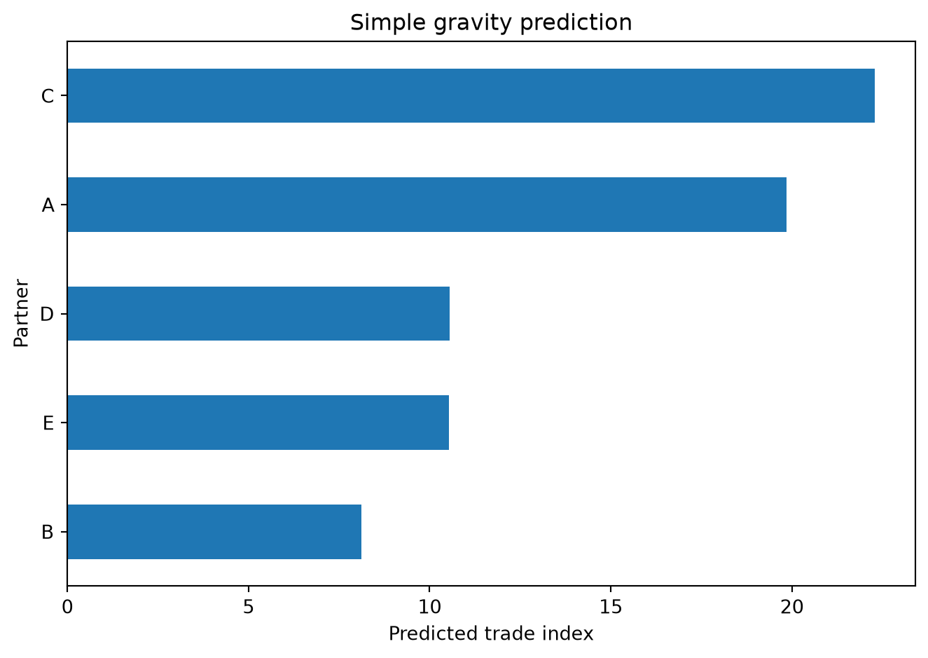
Python application: simple gravity predictions
The following example uses artificial data to show how a gravity-style model works. The numbers are not real trade data. They are only for teaching.
A positive RTA coefficient does not automatically prove that the agreement caused all extra trade. Good empirical work must think about timing, country-pair characteristics, omitted variables, and whether the agreement was created between countries that already traded heavily.
Application to Oman
The gravity model is useful for thinking about Oman’s trade partners.
Oman may trade more with countries that are:
geographically close,
economically large,
connected through ports and logistics networks,
part of regional supply chains,
linked by trade agreements,
major importers of energy or petrochemical products,
important suppliers of food, machinery, vehicles, or intermediate goods.
For Oman, gravity logic helps explain why regional partners matter, but it also leaves room for distant large economies such as China, India, the European Union, and the United States.
Gravity model and the final project
In student FTA projects, gravity logic helps interpret simulation results.
When you analyze a possible FTA, ask:
Are the countries economically large enough to generate meaningful trade?
Are they close enough for transport costs to be manageable?
Are they already trading with each other?
Are there major tariffs or non-tariff barriers that the FTA can reduce?
Are the countries complementary in production and demand?
Is the simulated trade increase likely to be trade creation or trade diversion?
These questions connect the gravity model to Chapters 8, 12, and 13.
Key takeaway
The gravity model predicts that bilateral trade is larger when countries are economically large and smaller when trade costs are high. GDP, distance, language, borders, infrastructure, tariffs, and RTAs help explain trade patterns.
The model is simple, but it is powerful because it connects trade theory to observable data. It also gives students a practical way to interpret country-pair trade and FTA simulation results.
Review questions
What is the basic intuition of the gravity model of trade?
Why does GDP increase predicted trade?
Why does distance reduce predicted trade?
Give three examples of trade-cost variables.
Why can a nearby smaller economy trade more than a distant larger economy?
How can a gravity model be used to study RTAs?
Why does a positive RTA coefficient not automatically prove welfare gains?
Why are agricultural products sensitive to trade facilitation?
How does the gravity model help interpret TINA simulation results?
What are two gravity-based reasons Oman may trade strongly with nearby partners?
Practice problem
Suppose Oman is comparing two potential trade partners.
Which partner has the higher predicted trade potential according to this simple score?
Explain why the larger economy does not necessarily have the higher score.
Name two other variables that a fuller gravity model should include.
Explain how an FTA could change predicted trade between Oman and one of these partners.
Text size
Style
Source Code
---title: "10. The Gravity Model of Trade"---## Learning objectivesBy the end of this chapter, you should be able to:1. Explain the basic intuition of the gravity model of trade.2. Identify why GDP and distance matter for bilateral trade flows.3. Interpret the expected signs of common gravity variables.4. Explain how trade costs affect bilateral trade.5. Use a simple gravity-style equation to compare predicted trade across partners.6. Connect gravity logic to regional trade agreements and TINA-style FTA simulations.## Why this chapter mattersEarlier chapters explained why countries trade using comparative advantage, factor endowments, and welfare analysis. The gravity model asks a different but very practical question:**Why does a country trade more with some partners than others?**The answer is usually not only comparative advantage. Trade also depends on the size of the partner economy, distance, transport costs, common borders, language, institutions, tariffs, and regional agreements.For applied trade analysis, the gravity model is useful because it connects trade theory to observable country-pair data.## The basic ideaThe gravity model is inspired by Newton’s law of gravity. In physics, the attraction between two objects increases with their mass and decreases with distance.In trade economics, bilateral trade tends to increase with the economic size of the two countries and decrease with trade costs, especially distance.A simple gravity-style expression is:$$Trade_{ij} = A \frac{GDP_i^{\alpha} GDP_j^{\beta}}{Distance_{ij}^{\gamma}}$$where:- $Trade_{ij}$ is trade between country $i$ and country $j$,- $GDP_i$ is the economic size of country $i$,- $GDP_j$ is the economic size of country $j$,- $Distance_{ij}$ is distance between the countries,- $A$ is a scaling factor,- $\alpha$, $\beta$, and $\gamma$ are parameters.The basic prediction is simple:- larger economies trade more,- closer economies trade more,- higher trade costs reduce trade.## Log-linear gravity equationEmpirical gravity models are often written in log form:$$\ln Trade_{ij} = \beta_0 + \beta_1 \ln GDP_i + \beta_2 \ln GDP_j - \beta_3 \ln Distance_{ij} + u_{ij}$$The expected signs are:| Variable | Expected sign | Interpretation ||---|---:|---|| Exporter GDP | Positive | Larger exporters can supply more goods. || Importer GDP | Positive | Larger importers demand more goods. || Distance | Negative | Greater distance raises transport and information costs. |This simple equation can be extended by adding trade-cost variables.## Trade-cost variablesDistance is only one proxy for trade costs. Many other factors affect bilateral trade.| Variable | Expected effect on trade | Reason ||---|---:|---|| Common border | Positive | Transport and coordination costs are usually lower. || Common language | Positive | Information and contract costs are lower. || Historical or colonial links | Positive | Networks and institutions may already exist. || Common currency | Positive | Currency conversion and exchange-rate uncertainty are lower. || Better infrastructure | Positive | Goods move faster and more reliably. || Higher tariffs | Negative | Tariffs raise import prices. || Regional trade agreement | Usually positive for members | Preferential access lowers trade barriers. || Long border delays | Negative | Time costs reduce competitiveness, especially for perishable goods. |For agricultural trade, time and logistics are especially important. Fresh fruits, vegetables, fish, dairy products, and livestock products are more sensitive to delays than many durable manufactured goods.## Worked example: size versus distanceSuppose Oman is comparing two potential trading partners using a simplified gravity score:$$Gravity\ score = \frac{Partner\ GDP\ index}{Distance\ index}$$This is not a full empirical model. It is only a teaching example.| Partner | Partner GDP index | Distance index | Gravity score ||---|---:|---:|---:|| Partner A | 500 | 1,000 | 0.50 || Partner B | 1,000 | 5,000 | 0.20 |Partner B is economically larger, but it is much farther away. Partner A has the higher gravity score because distance reduces predicted trade.:::: {.callout-note}## InterpretationThe gravity model does not say countries only trade with nearby partners. It says that, other things equal, distance reduces trade. A very large distant economy can still be an important partner.::::## Gravity and regional trade agreementsGravity models are often used to study regional trade agreements.A simple empirical model may include an RTA dummy variable:$$RTA_{ij} =\begin{cases}1 & \text{if countries } i \text{ and } j \text{ are in the same trade agreement} \\0 & \text{otherwise}\end{cases}$$If the estimated coefficient on the RTA dummy is positive, members trade more with each other after controlling for GDP, distance, and other factors.However, higher intra-bloc trade does not automatically mean the agreement is welfare-improving. As Chapter 8 explained, an RTA can create trade or divert trade.| Finding | Possible interpretation ||---|---|| Intra-RTA trade rises and trade with outsiders also rises | Likely trade creation or broader integration. || Intra-RTA trade rises but imports from efficient outsiders fall | Possible trade diversion. || No clear change | The agreement may be shallow, poorly implemented, or already anticipated by traders. |## Gravity and trade facilitationGravity models are also used to study trade facilitation.Trade facilitation means making it easier, faster, and cheaper for goods to cross borders. It includes customs procedures, port efficiency, documentation, inspection, digital systems, and transport infrastructure.Border delays can reduce trade because they increase time costs. This is especially relevant for agricultural products that are perishable or time-sensitive.Examples include:- fresh fruits and vegetables,- fish and seafood,- dairy products,- live animals,- chilled meat,- flowers and nursery products.For these goods, trade costs are not only monetary. Time is also a trade cost.## Python application: simple gravity predictionsThe following example uses artificial data to show how a gravity-style model works. The numbers are not real trade data. They are only for teaching.```{python}#| label: tbl-gravity-example#| echo: trueimport pandas as pdimport numpy as nppartners = pd.DataFrame({"Partner": ["A", "B", "C", "D", "E"],"Partner_GDP_index": [500, 1000, 800, 300, 1500],"Distance_index": [1000, 5000, 2000, 800, 6000],"RTA": [1, 0, 1, 0, 0],"Common_language": [0, 0, 1, 0, 0]})partners["Simple_gravity_score"] = partners["Partner_GDP_index"] / partners["Distance_index"]partners```Now we can create a slightly richer gravity-style prediction. We use a simple log equation with assumed coefficients:$$\ln Trade = \beta_0 + \beta_1 \ln GDP - \beta_2 \ln Distance + \beta_3 RTA + \beta_4 Language$$```{python}#| label: calc-gravity-predictions#| echo: truebeta_0 =2.0beta_gdp =1.0beta_distance =0.8beta_rta =0.30beta_language =0.20partners["Predicted_log_trade"] = ( beta_0+ beta_gdp * np.log(partners["Partner_GDP_index"])- beta_distance * np.log(partners["Distance_index"])+ beta_rta * partners["RTA"]+ beta_language * partners["Common_language"])partners["Predicted_trade_index"] = np.exp(partners["Predicted_log_trade"])partners[["Partner", "Predicted_log_trade", "Predicted_trade_index"]]``````{python}#| label: fig-gravity-predictions#| fig-cap: "Predicted trade index from a simple gravity-style model using artificial data."#| fig-width: 7#| fig-height: 4#| fig-format: svg#| echo: trueimport matplotlib.pyplot as pltplot_data = partners.sort_values("Predicted_trade_index", ascending=True)ax = plot_data.plot( kind="barh", x="Partner", y="Predicted_trade_index", legend=False)ax.set_xlabel("Predicted trade index")ax.set_ylabel("Partner")ax.set_title("Simple gravity prediction")plt.tight_layout()plt.show()```## Interpreting dummy variablesIn a log-linear gravity model, dummy-variable coefficients are often interpreted as approximate percentage effects.For example, if the RTA coefficient is:$$\beta_{RTA} = 0.30$$then the exact percentage effect is:$$100 \times \left(e^{0.30} - 1\right) \approx 35\%$$This means that, other things equal, members of the same RTA are predicted to trade about 35 percent more with each other.```{python}#| label: calc-rta-effect#| echo: truerta_coefficient =0.30rta_percent_effect =100* (np.exp(rta_coefficient) -1)print(f"RTA effect = {rta_percent_effect:.1f}%")```:::: {.callout-warning}## Be carefulA positive RTA coefficient does not automatically prove that the agreement caused all extra trade. Good empirical work must think about timing, country-pair characteristics, omitted variables, and whether the agreement was created between countries that already traded heavily.::::## Application to OmanThe gravity model is useful for thinking about Oman’s trade partners.Oman may trade more with countries that are:- geographically close,- economically large,- connected through ports and logistics networks,- part of regional supply chains,- linked by trade agreements,- major importers of energy or petrochemical products,- important suppliers of food, machinery, vehicles, or intermediate goods.For Oman, gravity logic helps explain why regional partners matter, but it also leaves room for distant large economies such as China, India, the European Union, and the United States.## Gravity model and the final projectIn student FTA projects, gravity logic helps interpret simulation results.When you analyze a possible FTA, ask:1. Are the countries economically large enough to generate meaningful trade?2. Are they close enough for transport costs to be manageable?3. Are they already trading with each other?4. Are there major tariffs or non-tariff barriers that the FTA can reduce?5. Are the countries complementary in production and demand?6. Is the simulated trade increase likely to be trade creation or trade diversion?These questions connect the gravity model to Chapters 8, 12, and 13.## Key takeawayThe gravity model predicts that bilateral trade is larger when countries are economically large and smaller when trade costs are high. GDP, distance, language, borders, infrastructure, tariffs, and RTAs help explain trade patterns.The model is simple, but it is powerful because it connects trade theory to observable data. It also gives students a practical way to interpret country-pair trade and FTA simulation results.## Review questions1. What is the basic intuition of the gravity model of trade?2. Why does GDP increase predicted trade?3. Why does distance reduce predicted trade?4. Give three examples of trade-cost variables.5. Why can a nearby smaller economy trade more than a distant larger economy?6. How can a gravity model be used to study RTAs?7. Why does a positive RTA coefficient not automatically prove welfare gains?8. Why are agricultural products sensitive to trade facilitation?9. How does the gravity model help interpret TINA simulation results?10. What are two gravity-based reasons Oman may trade strongly with nearby partners?## Practice problemSuppose Oman is comparing two potential trade partners.| Partner | GDP index | Distance index ||---|---:|---:|| Partner X | 900 | 3,000 || Partner Y | 400 | 800 |Use the simple gravity score:$$Gravity\ score = \frac{GDP\ index}{Distance\ index}$$1. Calculate the gravity score for each partner.2. Which partner has the higher predicted trade potential according to this simple score?3. Explain why the larger economy does not necessarily have the higher score.4. Name two other variables that a fuller gravity model should include.5. Explain how an FTA could change predicted trade between Oman and one of these partners.