04. Gains from Trade and Partial Equilibrium

Learning objectives

By the end of this chapter, you should be able to:

Explain consumer surplus, producer surplus, and total surplus.
Use a partial-equilibrium model to analyze one market.
Distinguish between autarky and free trade outcomes.
Identify which country exports and which country imports.
Derive excess supply and excess demand curves.
Calculate welfare changes from trade.
Use Python to compute and visualize trade equilibria.

Why this chapter matters

Trade changes prices. When prices change, some groups gain and some groups lose. Consumers, producers, and governments are affected differently.

Partial-equilibrium analysis helps us study these effects in one market at a time. This is useful for agricultural trade because many policy debates focus on specific products such as wheat, rice, milk, beef, fish, dates, or fertilizer.

The main lesson is simple: trade usually increases total surplus, but the gains are not distributed equally.

Partial equilibrium

A partial-equilibrium model studies one market while holding other markets constant.

For example, we may study the wheat market without modeling all other food markets. This is not a complete picture of the whole economy, but it is a useful way to understand the direct welfare effects of trade and trade policy.

In this chapter we use linear demand and supply curves:

\[ Q_d = a - bP \]

\[ Q_s = c + dP \]

where:

$Q_d$ is quantity demanded
$Q_s$ is quantity supplied
$P$ is price
$a$ and $c$ are intercept parameters
$b$ and $d$ are slope parameters

For most examples in this chapter, supply starts from the origin, so $c=0$.

Consumer surplus

Consumer surplus measures the difference between what consumers are willing to pay and what they actually pay.

Graphically, consumer surplus is the area below the demand curve and above the market price.

For a linear demand curve, if the choke price is $P_{\max}$, market price is $P$, and quantity demanded is $Q_d$, then:

\[ CS = \frac{1}{2}(P_{\max} - P)Q_d \]

The choke price is the price at which quantity demanded becomes zero.

Producer surplus

Producer surplus measures the difference between the price producers receive and the minimum price they would have accepted.

Graphically, producer surplus is the area above the supply curve and below the market price.

If supply starts from the origin, then:

\[ PS = \frac{1}{2}PQ_s \]

where $P$ is the market price and $Q_s$ is quantity supplied.

Total surplus

Total surplus is the sum of consumer surplus and producer surplus:

\[ TS = CS + PS \]

Total surplus is a simple measure of market welfare. It does not tell us whether the distribution of gains is fair, but it helps us measure whether the market as a whole gains or loses.

Important distinction

Trade can increase total surplus while reducing the surplus of one group.

For example, in an exporting country, producers may gain from a higher world price, while consumers lose because they pay more.

Autarky

Autarky means no trade.

In autarky, the domestic price is determined by domestic demand and domestic supply:

\[ Q_d = Q_s \]

If the autarky price is lower than the world price, the country tends to export under free trade.

If the autarky price is higher than the world price, the country tends to import under free trade.

Exporting country under free trade

An exporting country has a relatively low autarky price. When it opens to trade, the domestic price rises toward the world price.

Effects in the exporting country:

Group	Effect
Producers	Gain because they receive a higher price
Consumers	Lose because they pay a higher price
Total surplus	Usually increases

The country exports the difference between domestic quantity supplied and domestic quantity demanded:

\[ X = Q_s - Q_d \]

Importing country under free trade

An importing country has a relatively high autarky price. When it opens to trade, the domestic price falls toward the world price.

Effects in the importing country:

Group	Effect
Consumers	Gain because they pay a lower price
Producers	Lose because they receive a lower price
Total surplus	Usually increases

The country imports the difference between domestic quantity demanded and domestic quantity supplied:

\[ M = Q_d - Q_s \]

Excess supply and excess demand

To find the world price between two countries, we can use excess supply and excess demand.

For the exporting country:

\[ ES(P) = Q_s(P) - Q_d(P) \]

For the importing country:

\[ ED(P) = Q_d(P) - Q_s(P) \]

The world price is found where:

\[ ES(P) = ED(P) \]

This means that the quantity one country wants to export equals the quantity the other country wants to import.

Worked example: two-country trade

Suppose there are two countries and one good.

Country 1:

\[ Q_{d1} = 80 - P \]

\[ Q_{s1} = P \]

Country 2:

\[ Q_{d2} = 100 - 0.5P \]

\[ Q_{s2} = 0.5P \]

We will calculate:

Autarky equilibrium in each country.
Free-trade world price.
Consumer surplus, producer surplus, and total surplus.
The effect of a supply shock in Country 1.

Step 1: autarky equilibrium

In autarky, each country solves:

\[ Q_d = Q_s \]

Country 1

\[ 80 - P = P \]

\[ 2P = 80 \]

\[ P_1 = 40 \]

\[ Q_1 = 40 \]

Country 1 consumer surplus:

\[ CS_1 = \frac{1}{2}(80 - 40)(40) = 800 \]

Country 1 producer surplus:

\[ PS_1 = \frac{1}{2}(40)(40) = 800 \]

So:

\[ TS_1 = 1600 \]

Country 2

\[ 100 - 0.5P = 0.5P \]

\[ P_2 = 100 \]

\[ Q_2 = 50 \]

Country 2 demand has a choke price of 200 because:

\[ 100 - 0.5P = 0 \]

\[ P = 200 \]

Country 2 consumer surplus:

\[ CS_2 = \frac{1}{2}(200 - 100)(50) = 2500 \]

Country 2 producer surplus:

\[ PS_2 = \frac{1}{2}(100)(50) = 2500 \]

So:

\[ TS_2 = 5000 \]

Autarky summary

Country	Price	Quantity	CS	PS	TS
Country 1	40	40	800	800	1600
Country 2	100	50	2500	2500	5000
World total					6600

Country 1 has the lower autarky price, so it will export under free trade. Country 2 has the higher autarky price, so it will import.

Step 2: free-trade world price

Country 1 excess supply:

\[ ES_1(P) = Q_{s1} - Q_{d1} \]

\[ ES_1(P) = P - (80 - P) \]

\[ ES_1(P) = 2P - 80 \]

Country 2 excess demand:

\[ ED_2(P) = Q_{d2} - Q_{s2} \]

\[ ED_2(P) = (100 - 0.5P) - 0.5P \]

\[ ED_2(P) = 100 - P \]

Set excess supply equal to excess demand:

\[ 2P - 80 = 100 - P \]

\[ 3P = 180 \]

\[ P^* = 60 \]

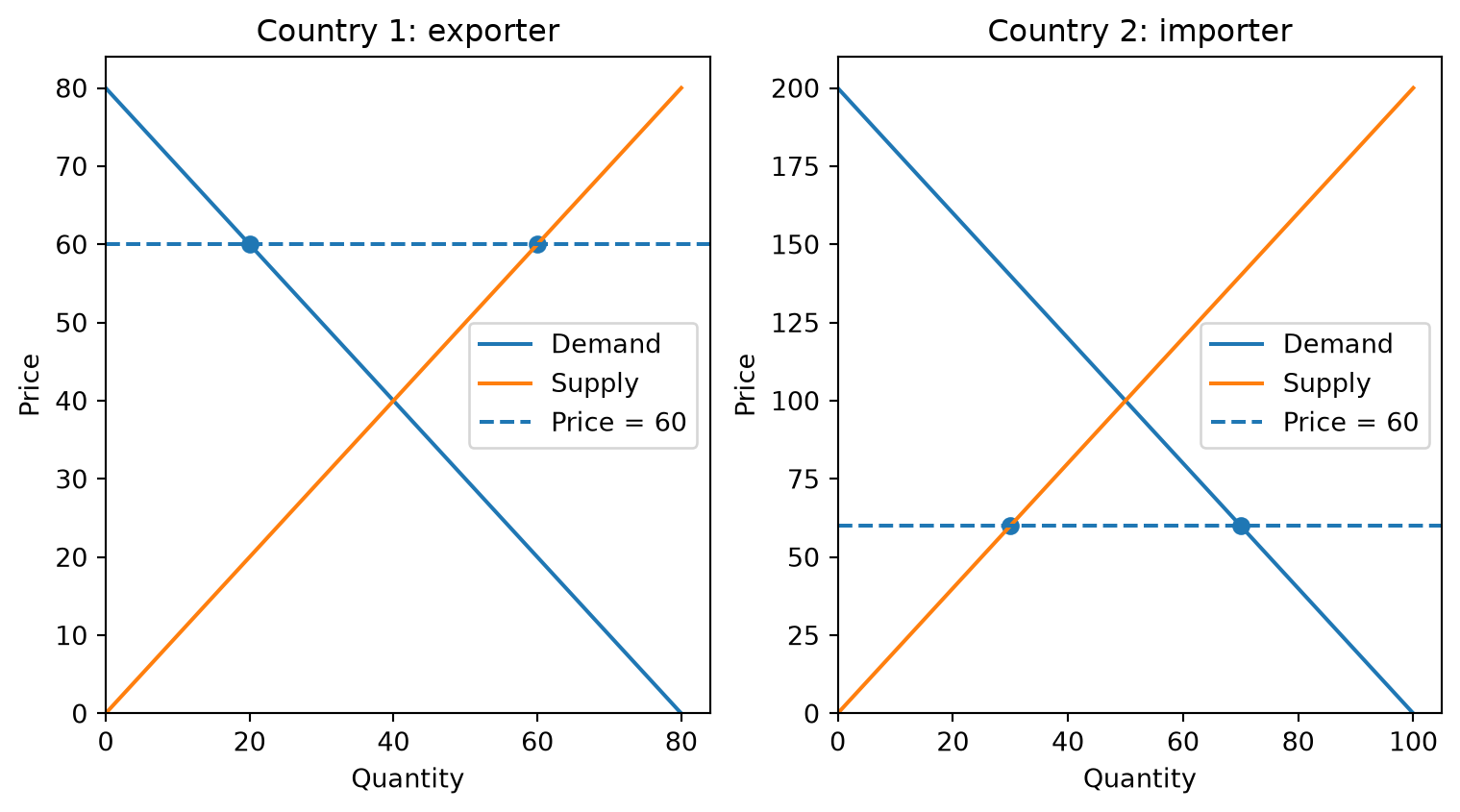
At $P^*=60$:

Country 1:

\[ Q_{d1} = 80 - 60 = 20 \]

\[ Q_{s1} = 60 \]

\[ X_1 = 60 - 20 = 40 \]

Country 2:

\[ Q_{d2} = 100 - 0.5(60) = 70 \]

\[ Q_{s2} = 0.5(60) = 30 \]

\[ M_2 = 70 - 30 = 40 \]

Exports equal imports, so the world market clears.

Step 3: welfare under free trade

Country 1: exporter

Country 1 consumer surplus falls:

\[ CS_1 = \frac{1}{2}(80 - 60)(20) = 200 \]

Country 1 producer surplus rises:

\[ PS_1 = \frac{1}{2}(60)(60) = 1800 \]

So:

\[ TS_1 = 2000 \]

Country 1 gains:

\[ \Delta TS_1 = 2000 - 1600 = 400 \]

Country 2: importer

Country 2 consumer surplus rises:

\[ CS_2 = \frac{1}{2}(200 - 60)(70) = 4900 \]

Country 2 producer surplus falls:

\[ PS_2 = \frac{1}{2}(60)(30) = 900 \]

So:

\[ TS_2 = 5800 \]

Country 2 gains:

\[ \Delta TS_2 = 5800 - 5000 = 800 \]

Free-trade summary

Country	World price	Qd	Qs	Trade	CS	PS	TS
Country 1	60	20	60	Exports 40	200	1800	2000
Country 2	60	70	30	Imports 40	4900	900	5800
World total				40 traded			7800

World total surplus increases:

\[ 7800 - 6600 = 1200 \]

Interpretation

Free trade raises total surplus in both countries, but it changes the distribution of surplus.

Country 1 producers gain, while Country 1 consumers lose. Country 2 consumers gain, while Country 2 producers lose.

Step 4: supply shock in the exporting country

Now suppose Country 1 experiences a negative supply shock. Its supply becomes:

\[ Q_{s1}^{new} = 0.5P \]

Country 1 excess supply becomes:

\[ ES_1^{new}(P) = 0.5P - (80 - P) \]

\[ ES_1^{new}(P) = 1.5P - 80 \]

Country 2 excess demand is unchanged:

\[ ED_2(P) = 100 - P \]

Set new excess supply equal to excess demand:

\[ 1.5P - 80 = 100 - P \]

\[ 2.5P = 180 \]

\[ P^* = 72 \]

At $P^*=72$:

Country 1:

\[ Q_{d1} = 80 - 72 = 8 \]

\[ Q_{s1}^{new} = 0.5(72) = 36 \]

\[ X_1 = 36 - 8 = 28 \]

Country 2:

\[ Q_{d2} = 100 - 0.5(72) = 64 \]

\[ Q_{s2} = 0.5(72) = 36 \]

\[ M_2 = 64 - 36 = 28 \]

The shock raises the world price from 60 to 72 and reduces trade volume from 40 to 28.

Welfare after the supply shock

Country 1:

\[ CS_1 = \frac{1}{2}(80 - 72)(8) = 32 \]

\[ PS_1 = \frac{1}{2}(72)(36) = 1296 \]

\[ TS_1 = 1328 \]

Country 2:

\[ CS_2 = \frac{1}{2}(200 - 72)(64) = 4096 \]

\[ PS_2 = \frac{1}{2}(72)(36) = 1296 \]

\[ TS_2 = 5392 \]

Country	World price	Qd	Qs	Trade	CS	PS	TS
Country 1	72	8	36	Exports 28	32	1296	1328
Country 2	72	64	36	Imports 28	4096	1296	5392
World total				28 traded			6720

The supply shock reduces world total surplus:

\[ 6720 - 7800 = -1080 \]

Python application

The Python code below calculates the same results and creates simple visualizations.

Code

import numpy as np
import pandas as pd
import matplotlib.pyplot as plt

def surplus_linear_demand_supply(a, b, d, price):
    """
    Demand: Qd = a - bP
    Supply: Qs = dP
    """
    qd = a - b * price
    qs = d * price
    p_max = a / b

    cs = 0.5 * (p_max - price) * qd
    ps = 0.5 * price * qs
    ts = cs + ps

    return {
        "Price": price,
        "Qd": qd,
        "Qs": qs,
        "CS": cs,
        "PS": ps,
        "TS": ts
    }

Code

country1_autarky = surplus_linear_demand_supply(a=80, b=1, d=1, price=40)
country2_autarky = surplus_linear_demand_supply(a=100, b=0.5, d=0.5, price=100)

autarky = pd.DataFrame(
    [country1_autarky, country2_autarky],
    index=["Country 1", "Country 2"]
)

autarky

	Price	Qd	Qs	CS	PS	TS
Country 1	40	40.0	40.0	800.0	800.0	1600.0
Country 2	100	50.0	50.0	2500.0	2500.0	5000.0

Code

country1_trade = surplus_linear_demand_supply(a=80, b=1, d=1, price=60)
country2_trade = surplus_linear_demand_supply(a=100, b=0.5, d=0.5, price=60)

free_trade = pd.DataFrame(
    [country1_trade, country2_trade],
    index=["Country 1", "Country 2"]
)

free_trade["Trade"] = free_trade["Qs"] - free_trade["Qd"]
free_trade

	Price	Qd	Qs	CS	PS	TS	Trade
Country 1	60	20.0	60.0	200.0	1800.0	2000.0	40.0
Country 2	60	70.0	30.0	4900.0	900.0	5800.0	-40.0

Code

def plot_country_market(ax, a, b, d, price, title):
    p_max = a / b
    p_values = np.linspace(0, p_max, 200)
    qd_values = a - b * p_values
    qs_values = d * p_values

    qd_price = a - b * price
    qs_price = d * price

    ax.plot(qd_values, p_values, label="Demand")
    ax.plot(qs_values, p_values, label="Supply")
    ax.axhline(price, linestyle="--", label=f"Price = {price:.0f}")
    ax.scatter([qd_price, qs_price], [price, price])
    ax.set_title(title)
    ax.set_xlabel("Quantity")
    ax.set_ylabel("Price")
    ax.set_xlim(left=0)
    ax.set_ylim(bottom=0)
    ax.legend()

fig, axes = plt.subplots(1, 2, figsize=(8, 4.5))

plot_country_market(
    axes[0],
    a=80,
    b=1,
    d=1,
    price=60,
    title="Country 1: exporter"
)

plot_country_market(
    axes[1],
    a=100,
    b=0.5,
    d=0.5,
    price=60,
    title="Country 2: importer"
)

plt.tight_layout()
plt.show()

Figure 7.1: Free trade raises the price in the exporting country and lowers the price in the importing country.

Code

country1_shock = surplus_linear_demand_supply(a=80, b=1, d=0.5, price=72)
country2_shock = surplus_linear_demand_supply(a=100, b=0.5, d=0.5, price=72)

shock = pd.DataFrame(
    [country1_shock, country2_shock],
    index=["Country 1", "Country 2"]
)

shock["Trade"] = shock["Qs"] - shock["Qd"]
shock

	Price	Qd	Qs	CS	PS	TS	Trade
Country 1	72	8.0	36.0	32.0	1296.0	1328.0	28.0
Country 2	72	64.0	36.0	4096.0	1296.0	5392.0	-28.0

Code

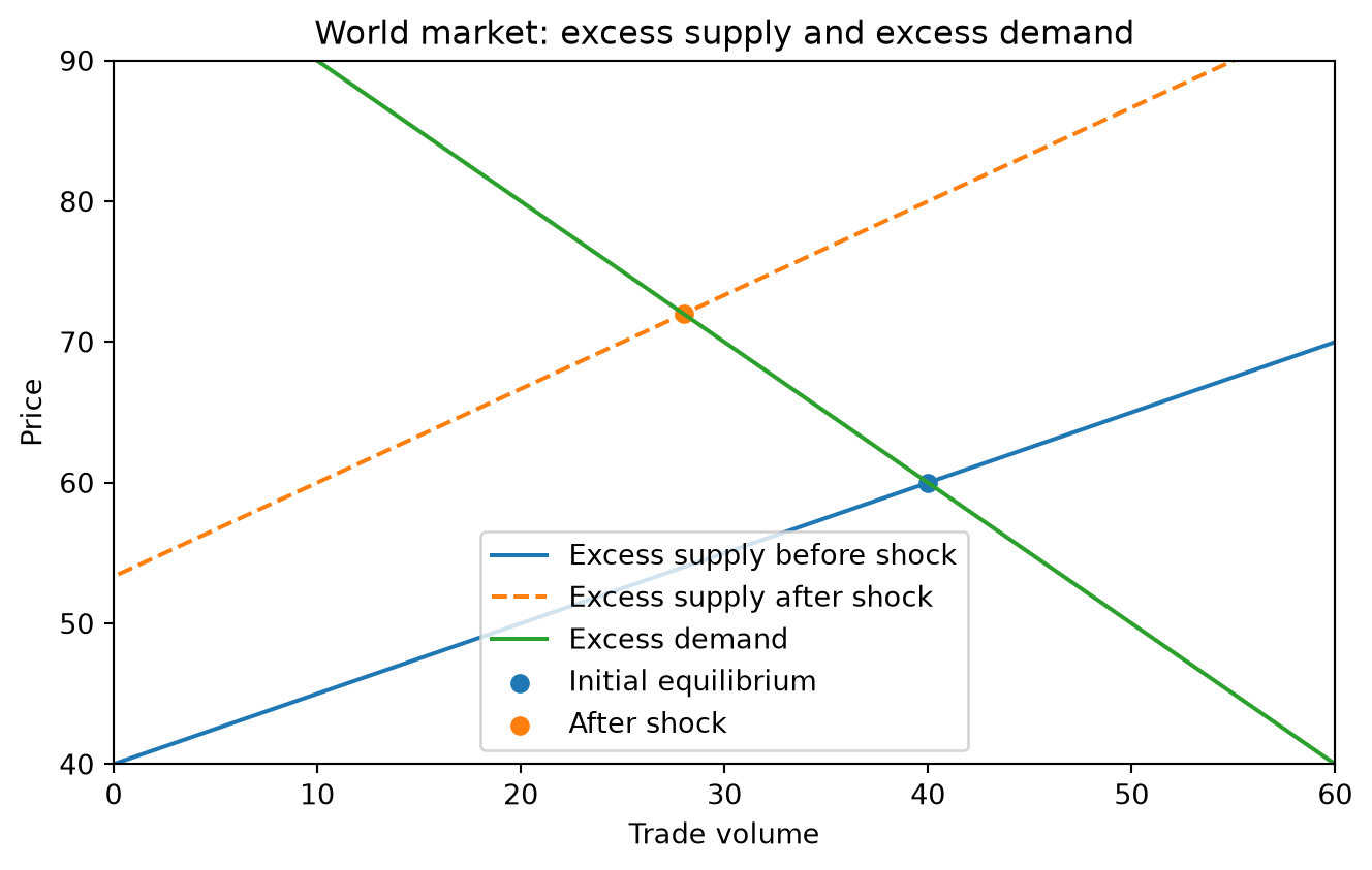
p = np.linspace(40, 90, 200)

es_before = 2 * p - 80
es_after = 1.5 * p - 80
ed = 100 - p

plt.figure(figsize=(7, 4.5))
plt.plot(es_before, p, label="Excess supply before shock")
plt.plot(es_after, p, linestyle="--", label="Excess supply after shock")
plt.plot(ed, p, label="Excess demand")

plt.scatter([40], [60], label="Initial equilibrium")
plt.scatter([28], [72], label="After shock")

plt.xlabel("Trade volume")
plt.ylabel("Price")
plt.title("World market: excess supply and excess demand")
plt.xlim(0, 60)
plt.ylim(40, 90)
plt.legend()
plt.tight_layout()
plt.show()

Figure 7.2: The supply shock reduces export supply, raises the world price, and lowers trade volume.

What the Python results show

The tables and figures confirm the analytical results.

Before trade, Country 1 has a lower price than Country 2. Therefore, Country 1 becomes the exporter and Country 2 becomes the importer.

Under free trade, world price becomes 60 and trade volume is 40. World total surplus increases.

After the negative supply shock in Country 1, the world price rises to 72 and trade volume falls to 28. This reduces total welfare relative to the original free-trade outcome.

Key takeaway

Partial-equilibrium analysis shows how trade changes prices, quantities, and welfare in one market.

The country with the lower autarky price exports. The country with the higher autarky price imports. Free trade usually increases total surplus, but it creates distributional conflict because consumers and producers are affected differently.

Review questions

What is consumer surplus?
What is producer surplus?
Why is total surplus equal to consumer surplus plus producer surplus?
What does autarky mean?
How do we identify the exporting country using autarky prices?
What is excess supply?
What is excess demand?
Why does the exporting country’s price rise under free trade?
Why does the importing country’s price fall under free trade?
How can trade increase total surplus while hurting one group?

Practice problem

Suppose Country A has:

\[ Q_d = 120 - 2P \]

\[ Q_s = 2P \]

Country B has:

\[ Q_d = 150 - P \]

\[ Q_s = P \]

Answer the following:

Find the autarky price and quantity in each country.
Identify which country will export and which country will import.
Derive the excess supply curve for the exporter.
Derive the excess demand curve for the importer.
Find the free-trade world price.
Calculate trade volume.
Explain which group gains and which group loses in each country.

--- title: "04. Gains from Trade and Partial Equilibrium" --- ## Learning objectives By the end of this chapter, you should be able to: 1. Explain consumer surplus, producer surplus, and total surplus. 2. Use a partial-equilibrium model to analyze one market. 3. Distinguish between autarky and free trade outcomes. 4. Identify which country exports and which country imports. 5. Derive excess supply and excess demand curves. 6. Calculate welfare changes from trade. 7. Use Python to compute and visualize trade equilibria. ## Why this chapter matters Trade changes prices. When prices change, some groups gain and some groups lose. Consumers, producers, and governments are affected differently. Partial-equilibrium analysis helps us study these effects in one market at a time. This is useful for agricultural trade because many policy debates focus on specific products such as wheat, rice, milk, beef, fish, dates, or fertilizer. The main lesson is simple: trade usually increases total surplus, but the gains are not distributed equally. ## Partial equilibrium A **partial-equilibrium model** studies one market while holding other markets constant. For example, we may study the wheat market without modeling all other food markets. This is not a complete picture of the whole economy, but it is a useful way to understand the direct welfare effects of trade and trade policy. In this chapter we use linear demand and supply curves: $$ Q_d = a - bP $$ $$ Q_s = c + dP $$ where: - $Q_d$ is quantity demanded - $Q_s$ is quantity supplied - $P$ is price - $a$ and $c$ are intercept parameters - $b$ and $d$ are slope parameters For most examples in this chapter, supply starts from the origin, so $c=0$. ## Consumer surplus **Consumer surplus** measures the difference between what consumers are willing to pay and what they actually pay. Graphically, consumer surplus is the area below the demand curve and above the market price. For a linear demand curve, if the choke price is $P_{\max}$, market price is $P$, and quantity demanded is $Q_d$, then: $$ CS = \frac{1}{2}(P_{\max} - P)Q_d $$ The choke price is the price at which quantity demanded becomes zero. ## Producer surplus **Producer surplus** measures the difference between the price producers receive and the minimum price they would have accepted. Graphically, producer surplus is the area above the supply curve and below the market price. If supply starts from the origin, then: $$ PS = \frac{1}{2}PQ_s $$ where $P$ is the market price and $Q_s$ is quantity supplied. ## Total surplus Total surplus is the sum of consumer surplus and producer surplus: $$ TS = CS + PS $$ Total surplus is a simple measure of market welfare. It does not tell us whether the distribution of gains is fair, but it helps us measure whether the market as a whole gains or loses. :::: {.callout-note} ## Important distinction Trade can increase total surplus while reducing the surplus of one group. For example, in an exporting country, producers may gain from a higher world price, while consumers lose because they pay more. :::: ## Autarky **Autarky** means no trade. In autarky, the domestic price is determined by domestic demand and domestic supply: $$ Q_d = Q_s $$ If the autarky price is lower than the world price, the country tends to export under free trade. If the autarky price is higher than the world price, the country tends to import under free trade. ## Exporting country under free trade An exporting country has a relatively low autarky price. When it opens to trade, the domestic price rises toward the world price. Effects in the exporting country: | Group | Effect | |---|---| | Producers | Gain because they receive a higher price | | Consumers | Lose because they pay a higher price | | Total surplus | Usually increases | The country exports the difference between domestic quantity supplied and domestic quantity demanded: $$ X = Q_s - Q_d $$ ## Importing country under free trade An importing country has a relatively high autarky price. When it opens to trade, the domestic price falls toward the world price. Effects in the importing country: | Group | Effect | |---|---| | Consumers | Gain because they pay a lower price | | Producers | Lose because they receive a lower price | | Total surplus | Usually increases | The country imports the difference between domestic quantity demanded and domestic quantity supplied: $$ M = Q_d - Q_s $$ ## Excess supply and excess demand To find the world price between two countries, we can use excess supply and excess demand. For the exporting country: $$ ES(P) = Q_s(P) - Q_d(P) $$ For the importing country: $$ ED(P) = Q_d(P) - Q_s(P) $$ The world price is found where: $$ ES(P) = ED(P) $$ This means that the quantity one country wants to export equals the quantity the other country wants to import. ## Worked example: two-country trade Suppose there are two countries and one good. Country 1: $$ Q_{d1} = 80 - P $$ $$ Q_{s1} = P $$ Country 2: $$ Q_{d2} = 100 - 0.5P $$ $$ Q_{s2} = 0.5P $$ We will calculate: 1. Autarky equilibrium in each country. 2. Free-trade world price. 3. Consumer surplus, producer surplus, and total surplus. 4. The effect of a supply shock in Country 1. ## Step 1: autarky equilibrium In autarky, each country solves: $$ Q_d = Q_s $$ ### Country 1 $$ 80 - P = P $$ $$ 2P = 80 $$ $$ P_1 = 40 $$ $$ Q_1 = 40 $$ Country 1 consumer surplus: $$ CS_1 = \frac{1}{2}(80 - 40)(40) = 800 $$ Country 1 producer surplus: $$ PS_1 = \frac{1}{2}(40)(40) = 800 $$ So: $$ TS_1 = 1600 $$ ### Country 2 $$ 100 - 0.5P = 0.5P $$ $$ P_2 = 100 $$ $$ Q_2 = 50 $$ Country 2 demand has a choke price of 200 because: $$ 100 - 0.5P = 0 $$ $$ P = 200 $$ Country 2 consumer surplus: $$ CS_2 = \frac{1}{2}(200 - 100)(50) = 2500 $$ Country 2 producer surplus: $$ PS_2 = \frac{1}{2}(100)(50) = 2500 $$ So: $$ TS_2 = 5000 $$ ### Autarky summary | Country | Price | Quantity | CS | PS | TS | |---|---:|---:|---:|---:|---:| | Country 1 | 40 | 40 | 800 | 800 | 1600 | | Country 2 | 100 | 50 | 2500 | 2500 | 5000 | | World total | | | | | 6600 | Country 1 has the lower autarky price, so it will export under free trade. Country 2 has the higher autarky price, so it will import. ## Step 2: free-trade world price Country 1 excess supply: $$ ES_1(P) = Q_{s1} - Q_{d1} $$ $$ ES_1(P) = P - (80 - P) $$ $$ ES_1(P) = 2P - 80 $$ Country 2 excess demand: $$ ED_2(P) = Q_{d2} - Q_{s2} $$ $$ ED_2(P) = (100 - 0.5P) - 0.5P $$ $$ ED_2(P) = 100 - P $$ Set excess supply equal to excess demand: $$ 2P - 80 = 100 - P $$ $$ 3P = 180 $$ $$ P^* = 60 $$ At $P^*=60$: Country 1: $$ Q_{d1} = 80 - 60 = 20 $$ $$ Q_{s1} = 60 $$ $$ X_1 = 60 - 20 = 40 $$ Country 2: $$ Q_{d2} = 100 - 0.5(60) = 70 $$ $$ Q_{s2} = 0.5(60) = 30 $$ $$ M_2 = 70 - 30 = 40 $$ Exports equal imports, so the world market clears. ## Step 3: welfare under free trade ### Country 1: exporter Country 1 consumer surplus falls: $$ CS_1 = \frac{1}{2}(80 - 60)(20) = 200 $$ Country 1 producer surplus rises: $$ PS_1 = \frac{1}{2}(60)(60) = 1800 $$ So: $$ TS_1 = 2000 $$ Country 1 gains: $$ \Delta TS_1 = 2000 - 1600 = 400 $$ ### Country 2: importer Country 2 consumer surplus rises: $$ CS_2 = \frac{1}{2}(200 - 60)(70) = 4900 $$ Country 2 producer surplus falls: $$ PS_2 = \frac{1}{2}(60)(30) = 900 $$ So: $$ TS_2 = 5800 $$ Country 2 gains: $$ \Delta TS_2 = 5800 - 5000 = 800 $$ ### Free-trade summary | Country | World price | Qd | Qs | Trade | CS | PS | TS | |---|---:|---:|---:|---:|---:|---:|---:| | Country 1 | 60 | 20 | 60 | Exports 40 | 200 | 1800 | 2000 | | Country 2 | 60 | 70 | 30 | Imports 40 | 4900 | 900 | 5800 | | World total | | | | 40 traded | | | 7800 | World total surplus increases: $$ 7800 - 6600 = 1200 $$ :::: {.callout-important} ## Interpretation Free trade raises total surplus in both countries, but it changes the distribution of surplus. Country 1 producers gain, while Country 1 consumers lose. Country 2 consumers gain, while Country 2 producers lose. :::: ## Step 4: supply shock in the exporting country Now suppose Country 1 experiences a negative supply shock. Its supply becomes: $$ Q_{s1}^{new} = 0.5P $$ Country 1 excess supply becomes: $$ ES_1^{new}(P) = 0.5P - (80 - P) $$ $$ ES_1^{new}(P) = 1.5P - 80 $$ Country 2 excess demand is unchanged: $$ ED_2(P) = 100 - P $$ Set new excess supply equal to excess demand: $$ 1.5P - 80 = 100 - P $$ $$ 2.5P = 180 $$ $$ P^* = 72 $$ At $P^*=72$: Country 1: $$ Q_{d1} = 80 - 72 = 8 $$ $$ Q_{s1}^{new} = 0.5(72) = 36 $$ $$ X_1 = 36 - 8 = 28 $$ Country 2: $$ Q_{d2} = 100 - 0.5(72) = 64 $$ $$ Q_{s2} = 0.5(72) = 36 $$ $$ M_2 = 64 - 36 = 28 $$ The shock raises the world price from 60 to 72 and reduces trade volume from 40 to 28. ## Welfare after the supply shock Country 1: $$ CS_1 = \frac{1}{2}(80 - 72)(8) = 32 $$ $$ PS_1 = \frac{1}{2}(72)(36) = 1296 $$ $$ TS_1 = 1328 $$ Country 2: $$ CS_2 = \frac{1}{2}(200 - 72)(64) = 4096 $$ $$ PS_2 = \frac{1}{2}(72)(36) = 1296 $$ $$ TS_2 = 5392 $$ | Country | World price | Qd | Qs | Trade | CS | PS | TS | |---|---:|---:|---:|---:|---:|---:|---:| | Country 1 | 72 | 8 | 36 | Exports 28 | 32 | 1296 | 1328 | | Country 2 | 72 | 64 | 36 | Imports 28 | 4096 | 1296 | 5392 | | World total | | | | 28 traded | | | 6720 | The supply shock reduces world total surplus: $$ 6720 - 7800 = -1080 $$ ## Python application The Python code below calculates the same results and creates simple visualizations. ```{python} #| label: chp4-setup #| echo: true import numpy as np import pandas as pd import matplotlib.pyplot as plt def surplus_linear_demand_supply(a, b, d, price): """ Demand: Qd = a - bP Supply: Qs = dP """ qd = a - b * price qs = d * price p_max = a / b cs = 0.5 * (p_max - price) * qd ps = 0.5 * price * qs ts = cs + ps return { "Price": price, "Qd": qd, "Qs": qs, "CS": cs, "PS": ps, "TS": ts } ``` ```{python} #| label: chp4-autarky-table #| echo: true country1_autarky = surplus_linear_demand_supply(a=80, b=1, d=1, price=40) country2_autarky = surplus_linear_demand_supply(a=100, b=0.5, d=0.5, price=100) autarky = pd.DataFrame( [country1_autarky, country2_autarky], index=["Country 1", "Country 2"] ) autarky ``` ```{python} #| label: chp4-free-trade-table #| echo: true country1_trade = surplus_linear_demand_supply(a=80, b=1, d=1, price=60) country2_trade = surplus_linear_demand_supply(a=100, b=0.5, d=0.5, price=60) free_trade = pd.DataFrame( [country1_trade, country2_trade], index=["Country 1", "Country 2"] ) free_trade["Trade"] = free_trade["Qs"] - free_trade["Qd"] free_trade ``` ```{python} #| label: fig-chp4-free-trade #| fig-cap: "Free trade raises the price in the exporting country and lowers the price in the importing country." #| fig-width: 8 #| fig-height: 4.5 #| echo: true def plot_country_market(ax, a, b, d, price, title): p_max = a / b p_values = np.linspace(0, p_max, 200) qd_values = a - b * p_values qs_values = d * p_values qd_price = a - b * price qs_price = d * price ax.plot(qd_values, p_values, label="Demand") ax.plot(qs_values, p_values, label="Supply") ax.axhline(price, linestyle="--", label=f"Price = {price:.0f}") ax.scatter([qd_price, qs_price], [price, price]) ax.set_title(title) ax.set_xlabel("Quantity") ax.set_ylabel("Price") ax.set_xlim(left=0) ax.set_ylim(bottom=0) ax.legend() fig, axes = plt.subplots(1, 2, figsize=(8, 4.5)) plot_country_market( axes[0], a=80, b=1, d=1, price=60, title="Country 1: exporter" ) plot_country_market( axes[1], a=100, b=0.5, d=0.5, price=60, title="Country 2: importer" ) plt.tight_layout() plt.show() ``` ```{python} #| label: chp4-supply-shock-table #| echo: true country1_shock = surplus_linear_demand_supply(a=80, b=1, d=0.5, price=72) country2_shock = surplus_linear_demand_supply(a=100, b=0.5, d=0.5, price=72) shock = pd.DataFrame( [country1_shock, country2_shock], index=["Country 1", "Country 2"] ) shock["Trade"] = shock["Qs"] - shock["Qd"] shock ``` ```{python} #| label: fig-chp4-world-market #| fig-cap: "The supply shock reduces export supply, raises the world price, and lowers trade volume." #| fig-width: 7 #| fig-height: 4.5 #| echo: true p = np.linspace(40, 90, 200) es_before = 2 * p - 80 es_after = 1.5 * p - 80 ed = 100 - p plt.figure(figsize=(7, 4.5)) plt.plot(es_before, p, label="Excess supply before shock") plt.plot(es_after, p, linestyle="--", label="Excess supply after shock") plt.plot(ed, p, label="Excess demand") plt.scatter([40], [60], label="Initial equilibrium") plt.scatter([28], [72], label="After shock") plt.xlabel("Trade volume") plt.ylabel("Price") plt.title("World market: excess supply and excess demand") plt.xlim(0, 60) plt.ylim(40, 90) plt.legend() plt.tight_layout() plt.show() ``` ## What the Python results show The tables and figures confirm the analytical results. Before trade, Country 1 has a lower price than Country 2. Therefore, Country 1 becomes the exporter and Country 2 becomes the importer. Under free trade, world price becomes 60 and trade volume is 40. World total surplus increases. After the negative supply shock in Country 1, the world price rises to 72 and trade volume falls to 28. This reduces total welfare relative to the original free-trade outcome. ## Key takeaway Partial-equilibrium analysis shows how trade changes prices, quantities, and welfare in one market. The country with the lower autarky price exports. The country with the higher autarky price imports. Free trade usually increases total surplus, but it creates distributional conflict because consumers and producers are affected differently. ## Review questions 1. What is consumer surplus? 2. What is producer surplus? 3. Why is total surplus equal to consumer surplus plus producer surplus? 4. What does autarky mean? 5. How do we identify the exporting country using autarky prices? 6. What is excess supply? 7. What is excess demand? 8. Why does the exporting country’s price rise under free trade? 9. Why does the importing country’s price fall under free trade? 10. How can trade increase total surplus while hurting one group? ## Practice problem Suppose Country A has: $$ Q_d = 120 - 2P $$ $$ Q_s = 2P $$ Country B has: $$ Q_d = 150 - P $$ $$ Q_s = P $$ Answer the following: 1. Find the autarky price and quantity in each country. 2. Identify which country will export and which country will import. 3. Derive the excess supply curve for the exporter. 4. Derive the excess demand curve for the importer. 5. Find the free-trade world price. 6. Calculate trade volume. 7. Explain which group gains and which group loses in each country.